library(readr)

day1_data <- read_delim(file = "./data/Day1.txt", delim = "/t",
                        col_names = "depth", show_col_types = FALSE)

head(day1_data)
# A tibble: 6 × 1
depth
<dbl>
1 191
2 185
3 188
4 189
5 204
6 213It’s that time of year again. Houses are lit up, presents are being bought, and Michael Bublé has emerged from his hibernation to create another album of Christmas songs. This year, in the spirit of giving, I will share my code for the 2021 Advent of Code challenges. Each day is a new small coding challenge and I’ll attempt to upload and explain all my solutions! If I miss posting on any days (or you just want to look at the code in more detail) check out my GitHub repo.

We are given a numeric vector containing values of ocean depth. I’ll read it in as a data frame here.
library(readr)
day1_data <- read_delim(file = "./data/Day1.txt", delim = "/t",
col_names = "depth", show_col_types = FALSE)
head(day1_data)# A tibble: 6 × 1
depth
<dbl>
1 191
2 185
3 188
4 189
5 204
6 213For the first challenge we need to compare values along a vector and determine whether they increase or decrease. We then need to determine the number of times the depth value has increased (i.e. ocean floor became deeper). This one’s pretty straight forward, as we can just use the lead() function from dplyr to compare our vector of depths to its neighbour.
#Each value in the vector is compared to its neighbour. Return logical to check whether depth has increased
logical_output <- day1_data$depth < lead(day1_data$depth)

#Example output
logical_output[1:10]
[1] FALSE TRUE TRUE TRUE TRUE TRUE TRUE FALSE FALSE TRUE#Final result
sum(logical_output, na.rm = TRUE)[1] 1709For the second challenge we need to first create a new vector using a sliding window of size 3 (the sum of each value and its next two neighbours). Then we make the same check to see how often depth has increased using this newly created vector. This isn’t too much harder as we can use the n argument in lead() to return the 1st and 2nd neighbours.
#Create sliding window vector with window size 3
new_vector <- day1_data$depth + lead(day1_data$depth, n = 1) + lead(day1_data$depth, n = 2)
sum(new_vector < lead(new_vector), na.rm = TRUE)
[1] 1761This works, but this type of code always feels a bit inflexible to me. What if needed to change the size of the window? We would need to re-write our definition of new_vector every time. What if the size of the sliding window becomes very large? The definition for new_vector would also become very long and difficult to follow. Is there a functional way we can deal with this?
Firstly, I’ll consider an approach using the tidyverse where I work in a data frame. I create a loop with purrr to add any number of new columns each with a different lead value. You might notice the walrus operator (:=) which is used in the tidyverse to create dynamic column names. I then use the package lay and its eponymous function to efficiently apply a function (sum()) across rows of a data frame. You’ll need to install the lay package from GitHub.
#remotes::install_github("courtiol/lay")
library(lay)
library(purrr)

#Create a function that can take any window size
tidy_windowfunc <- function(data, window_size = 3){

  new_vector <- data %>%
    #Window includes the existing depth col, so we add window_size - 1 new columns
    mutate(map_dfc(.x = (1:window_size) - 1,
                   .f = function(i, depth){

                     #Create a new column with lag i
                     #Allow for dynamic col names
                     tibble("depth_lag{i}" := lead(depth, n = i))

                   }, depth = .data$depth)) %>%
    #Sum all the newly created lag columns using lay
    mutate(depth_sum = lay(across(.cols = contains("lag")), .fn = sum)) %>%
    pull(depth_sum)

  sum(new_vector < lead(new_vector), na.rm = TRUE)

}
Now we can solve both puzzles using just one function!
#Recreate Challenge 1
tidy_windowfunc(data = day1_data, window_size = 1) == sum(day1_data$depth < lead(day1_data$depth), na.rm = TRUE)
[1] TRUE#Recreate Challenge 2
new_vector <- day1_data$depth + lead(day1_data$depth, n = 1) + lead(day1_data$depth, n = 2)
tidy_windowfunc(data = day1_data, window_size = 3) == sum(new_vector < lead(new_vector), na.rm = TRUE)[1] TRUEThis was the tidyverse way, but can we do it any better using base R? My first thought here would be to try a while() loop, that continues adding new neighbours until window size is reached.
#Create similar function with base R
base_windowfunc <- function(data, window_size = 3){

  i <- 1
  depth      <- data$depth
  new_vector <- data$depth

  #As long as we haven't reached window size, keep going!
  while (i < window_size) {

    #Add depth data shifted by i to our existing vector.
    #Will ensure vectors are same length (adds NAs at the end)
    new_vector <- new_vector + depth[1:length(depth) + i]
    i <- i + 1

  }

  sum(new_vector[1:(length(new_vector) - 1)] < new_vector[2:length(new_vector)], na.rm = TRUE)

}
This works too and, as with most base R code, it’s 100% dependency free!
#Recreate Challenge 1
tidy_windowfunc(data = day1_data, window_size = 1) == base_windowfunc(data = day1_data, window_size = 1)
[1] TRUE#Recreate Challenge 2
tidy_windowfunc(data = day1_data, window_size = 3) == base_windowfunc(data = day1_data, window_size = 3)[1] TRUESo which one is faster? I would assume that by working exclusively with vectors our base R function will be faster than our tidy function that spends some time manipulating a data frame. Is this actually the case? And if so, how much faster do we get? Let’s look at the number of iterations/sec for each function and different window sizes using the mark() function in the bench package.
library(bench)

bench_df <- map_df(.x = 1:20,
                   .f = function(i){

                     times <- mark(tidy_windowfunc(data = day1_data, window_size = i),
                                   base_windowfunc(data = day1_data, window_size = i))

                     data.frame(method = c("tidy", "base"),
                                size = i,
                                number_per_sec = times$`itr/sec`,
                                speed_sec = 1/times$`itr/sec`)

                   })

ggplot(bench_df) +
  geom_line(aes(x = size, y = number_per_sec, colour = method), size = 1) +
  geom_point(aes(x = size, y = number_per_sec, colour = method), stroke = 1.5, shape = 21, fill = "white") +
  scale_y_continuous(name = "Iterations/sec",
                     breaks = seq(0, 15000, 5000), limits = c(0, 15000)) +
  scale_x_continuous(name = "Window size") +
  scale_colour_discrete(name = "") +
  labs(title = "Advent of Code Day 1",
       subtitle = "base v. tidyverse approach") +
  theme_classic(base_family = "Courier New") +
  theme(axis.text = element_text(colour = "black"),
        legend.position = c(0.8, 0.8),
        legend.background = element_rect(colour = "black"),
        legend.title = element_blank())
Warning: Using `size` aesthetic for lines was deprecated in ggplot2 3.4.0.
ℹ Please use `linewidth` instead.Warning: Removed 3 rows containing missing values (`geom_line()`).Warning: Removed 3 rows containing missing values (`geom_point()`).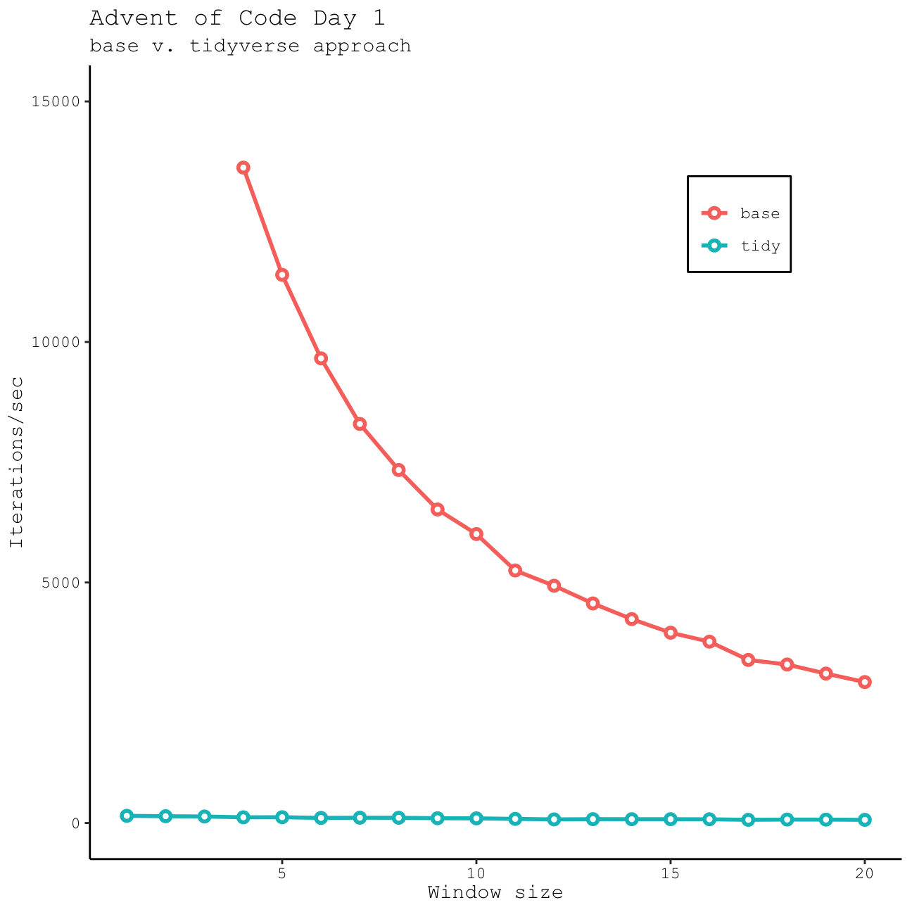
As expected, base R is more efficient, especially if we only need to work with short windows; however, this advantage decreases rapidly as we start to work with larger windows. Although it is slower, I think the tidyverse method I’ve used here is also very versatile, particularly if you want to return a data frame and not just a vector. Either way…they both get the correct result!